
Author: Mihai Avram | Date: 06/02/2021
Most people in tech know that Machine Learning is blowing up and that it can be applied in many different areas. This is a short guide for the specific context of applying Machine Learning to language. With enough curiosity in understanding the concepts and backlinks, it should robustly pass you over in the beginner phase of learning how to apply Machine Learning towards text.
Applying Machine Learning to text is a field which is also known as Natural Language Processing (NLP) or Computational Linguistics. We cover topics such as data gathering, data cleaning, supervised, unsupervised, and deep learning methods, as well as how to evaluate our models and apply them in the real world to solve classification, clustering problems, and more. Let’s dive in.
Input Data
In the the realm of NLP, without data, it is difficult to do exciting things. But what does the notion of data mean in this context? Simple, just text, and text labeled for various purposes. Let us say for example that we are building a classifier that can detect the gender of the subject in a given sentence. Here are two examples of one data point below, meant for this purpose:
Data Input:
“John went to the store to buy some apples, and brought them back home to his family a few hours later.”
Target Label:
“Male”
Data Input:
“Jane was recently promoted to a Senior Administrator position and she was thrilled!”
Target Label:
“Female”
Now for this classification problem we understand what data we need to feed the algorithm – but how much data? Certainly more than two data points, and it greatly depends on our context, problem we are trying to solve, structure of our data, and many other factors. The best way to answer it is to start with as much data as we can get, and try, with trial and error to see how our classifier is doing using the Evaluation methods explained later in this article. A general rule of thumb is that for supervised methods (e.g. Naive Bayes, Logistic Regression, etc.) we will need a lot less data than for Deep Learning methods (e.g. RNNs, Transformers, etc.).
We also have to pay attention to how we label our data, either manually, or finding a vendor that can do it for us. Some problems like in the gender example above, we have one input (a sentence) and one output label (the gender) which is a one-to-one mapping. Some NLP problems are more nuanced and may have an output of (true / false) in binary classification, or multi-label classification with many possible output options (e.g. options a, b, c, d, etc.).
Data Preprocessing
A machine or computer cannot just read text as it is like we can. Therefore, we typically need to preprocess our data. Supervised methods can especially benefit from this with one-hot encodings or word embeddings, which we will cover later. However, any other pre-processing steps you should try with a grain of salt on Deep Learning methods as they may not work. This is because Deep Learning methods understand a myriad of patterns from your data and sometimes non-pre-processed data can contain extra patterns the Deep Learning methods can pick up on, and by eliminating them, we could potentially remove those patterns. Here are some useful preprocessing steps.
Tokenization
We take a piece of text such as “John ate the apple.” and we split each token into an entity so that the rest of the process has the atomic components of the text to work with, such as “John” and “ate” and “the” and “.” at the end. These atomic components can really help in further downstream tasks when we have to normalize, or stem our data for instance.
Normalization
We also want to remove redundant items from our text such as extra spaces, stop words (which are common words like “the” or “to”), and any other irrelevant text components for the task at hand. Let’s say that you are parsing a web page and only need the paragraph from the first header, in such a case you want to remove any
html header tags from your text! Finally, we want to remove or replace unnecessary symbols such as accents (e.g. é should be converted to e and Ó to O).
Stemming and/or Lemmatization
This involves converting all words into their base form. There are many ways that one can convey a theme. For instance, the following two sentences:
“Jane liked skydiving”
“Jane likes skydiving”
These two sentences convey the same theme that Jane is enamored with skydiving, but at the bit-wise level and how the computer understands them, these two sentences are different. Once we lemmatize these two sentences, they will be lemmatized to something like “Jane like skydive” which applies to all versions of conveying this idea – and can really help downstream tasks such as classifiers better pick up on patterns.
What is the difference between stemming and lemmatization? In short, stemming creates a simple mapping between words and their root forms, while lemmatization considers word context in a sentence or phrase and can create root words based on more language and vocabulary factors instead of just a simple mapping. For more information on stemming and lemmatization, check out this resource.
Word Embeddings
The final step of our preprocessing involves turning all the text we have into vectors of numbers. Computers can only understand numbers, so this conversion must be done so that the NLP algorithms can work. An example of what this will look like is turning a sentence such as “Jane like skydive” to a list that resembles a unique number for each word.
["Jane like skydive"] -> [3, 5, 2]
Another way to build word embeddings is through one-hot encoding which is a mapping that presents all words in a corpus. For the purposes of highlighting this point, let’s say we have a corpus with only 3 words (though in the real world we will have corpora that easily span more than 10,000 words). The three words are “Jane”, “like” and “skydive”. We can then represent them as such:
"Jane" -> [1, 0, 0]
"like" -> [0, 1, 0]
"skydive" -> [0, 0, 1]
Where each word will have a 1 in a unique spot, and 0 everywhere else. There are many ways to build such embeddings, and each NLP framework will have its own methods. One popular method is using Word2Vec which maps each word in a high dimensional space so that the notion of how close, or far away, two words are – in meaning – can be showcased with vectors.
Here is a good resource explaining how Word2Vec works.
Other popular word embedding methods include TF-IDF, Glove, Fastext, and ELMO which you can learn more about here.
That’s about it for preprocessing! If you want to learn more about NLP Text Preprocessing and word embedding techniques, check out the following resources.
Supervised Methods for NLP
The most popular and easy to understand NLP methods are supervised learning methods. These consist of providing an NLP classifier preprocessed input data along with output data which is labeled.
Referring back to our Input Data section from above, we will need to provide the input data, and the outcomes of that data so that the algorithm can actually see how to correctly label automatically. Here are some popular and effective supervised learning methods:
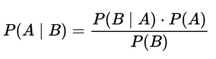
Naive Bayes – A simple method based on the Bayes’ Theorem that can help compute conditional probabilities based on occurrences of multiple events.
Pros:
– Easiest to implement
– Typically does not overfit (concept covered later)
– Easy to train
Cons:
– If you are working with data which has features that are dependent on each other, then it will perform poorly
– Can introduce bias from the features
For more information about Naive Bayes, see the following article called – A practical explanation of a Naive Bayes classifier
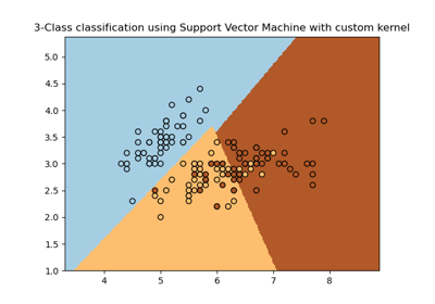
Support Vector Machines (SVMs) – Creates a boundary in some positive dimensional space (e.g. a line dividing two sides of a map) and uses that boundary to see what to label the input data. As an example, if a data point falls to the right of that boundary, perhaps the text is classified as spam. On the other hand, if it falls to the left of the boundary, the text is classified as non-spam.
Below is an example highlighting how an SVM can create decision boundaries to cluster different groups (blue, yellow, and red groups in this case which all make up different classes).
Pros:
– Works very well when one has a lot of features to work with
– Also performs well when there is a clear margin of separation between classes
Cons:
– Does not perform well when the data is noisy
– Not very well suited to large data sets
For more information about SVMs, see this article called – Text Classification Using Support Vector Machines (SVM)
Logistic Regression – A type of regression function that takes the output and passes it through a sigmoid function which transforms any number between 0 and 1 which can then be used to predict between two classes. If you have more classes to predict, Multinomial Logistic Regression will be your friend there.
For more information about Logistic Regression, see this article called – Build Your First Text Classifier in Python with Logistic Regression
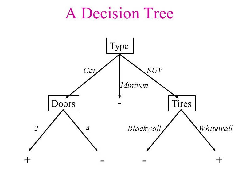
Decision Trees – Creates a system of decision rules as inferred from prior data samples. For instance, in the case of detecting spam, the algorithm may go through a series of questions, or decisions. Is the e-mail sent from an address that is from a blacklist? Does the e-mail contain a subject line? etc. Based on these decisions, and having seen many training data points with accurate labels (e.g. spam, non-spam), these decision boundaries are created and can best predict the problem at hand.
Below is an example of a decision tree that can predict types of cars based on their specs.
Pros:
– Easy to understand and explain
– Requires little to no preprocessing
Cons:
– Can be very volatile to data changes
– Takes a while to train the model
For more information about Decision Trees, check out this article – Decision Trees Explained Easily
Ensemble Methods for NLP
So we have all these methods and bags of tricks for solving Machine Learning problems. What if we could combine the results of all of them and create one aggregate result? That is the purpose of Ensemble Methods. They essentially combine the results of many classifiers in our toolkit (e.g. Logistic Regression, Naive Bayes, etc.) and use voting or averaging to come up with a one solution consensus. There are a few ways of doing this.
Voting
We create many learners which can just be the same algorithm trained on different data points, or different algorithms trained on the same data, or anything in between. Once we have all of these algorithms, we can have them vote what they yield as the correct prediction. We then tally up the votes and either pick the majority vote, or use some weighted scheme to find which prediction is true. Perhaps one of the algorithms you built has been vetted to be one the best-in-class for the prediction problem, so you give that algorithm a very high vote weight (e.g. the equivalent of 10 votes). This way the vote aggregation is done fairly based on the strength of the learners you have built. The same concept applies to regression, except for instead of tallying votes, one would average the results.
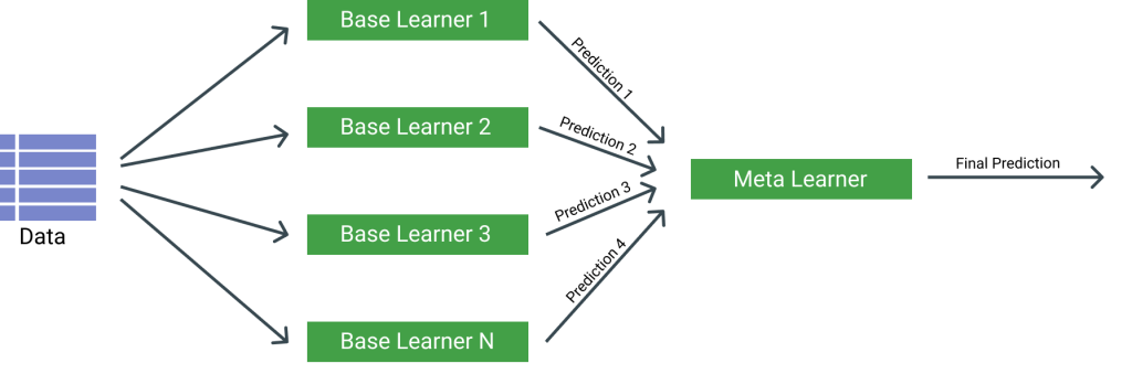
Stacking
In this case we create a classifier that can take our input data and have resulting predictions. Such predictions are then used for another classifier as input so that the encompassing classifier can make better predictions. One could imagine creating a stacked pipeline of many algorithms that feed their output to each other until a final classifier in the pipeline is able to predict the final labels. Something like the following diagram.
Bagging
Imagine having a dataset of 1,000 points. We can use bootstrap sampling where we can take random points from this dataset (some of them even double-counted) and create whole new subsets of this dataset. Using the many samples of data we created, we can then feed them as input to a classifier or group of classifiers and voting techniques will allow us to aggregate a result from all these methods. A popular and powerful Bagging method is Random Forest which uses Decision Trees as the base classifier.
Here’s a good resource to learn about Decision Trees and Random Forest.
Boosting
A family of classifiers that are able to convert weak machine learning algorithms together so that together they become strong. Any models that can perform a bit better than random guessing can become powerful if they are combined. These classifiers can be combined through a majority vote and one of the most popular and powerful methods for this is called AdaBoost.
Here’s a good resource to learn about AdaBoost.
One big caveat of ensemble methods is that they are not very interpretable. So even though you can write complex code and stack many algorithms to get the highest performance, you may not be able to explain your results so be wary of this when creating the classifiers. If your task at hand requires a lot of explainability and transparency, then ensemble methods may not be for you.
For a great resource describing ensemble methods, check out the following blog post from Toptal called Ensemble Methods: Elegant Techniques to Produce Improved Machine Learning Results
Unsupervised Methods for NLP
Unsupervised methods do not require any labeled data to ascertain patterns and find possible responses to our questions. The most popular unsupervised methods in NLP are clustering methods such as K-Means Clustering, or Latent Dirichlet Allocation (LDA). There is some complexity to these methods so we will briefly explain them and point to links that truly gives them justice.
K-Means Clustering
A method that groups input data together based on commonalities. Say that you have a large amount of text data that can either be labeled as spam or non-spam. Note that in this instance perhaps you don’t have any labels here because you never had time to manually look at each data point by hand and label it. No problem, K-Means will take your data points and find commonalities between them which will cluster the groups together in as many groups as you would like. In this case, let’s say we should only have a spam and non-spam group, so 2 groups in total. We then should only see the results being two grouped clusters cleanly divided into spam and non-spam. Note that there are many other Clustering techniques and K-Means is just one of them.
To learn more, you can check out this K-Means Clustering Resource.
Word2Vec
A very popular unsupervised method in NLP is Word2Vec. It works similar to clustering; however, imagine that each data point or word can stand on its own and has unique features about it. Word2Vec essentially coverts words into vectors – or numerical representations of a word. These representations allow various algorithms to find similarities between such vectors (e.g. the fact that dog and cat are both animals but a pencil is not). Using Word2Vec you can create a model that can tell the difference between words, among other things.
To learn more, you can check out this Word2Vec Resource.
Latent Dirichlet Allocation (LDA)
LDA is a method similar to K-Means clustering but focused on topic modeling text data. In particular it maps words to topics, and topics to documents. Note that a document here has a semantic meaning and it can really be just any text (e.g. a paragraph, a sentence, or a web page). LDA finds distributions of how these words, topics, and documents are related, and based on those distributions it can then create clusters of data from all of your text documents and be able to group them. An example of this is having 100 news articles spread out among 3 categories (sports, politics, and weather). After running LDA on our articles, we should be able to get back clearly divided sections where 20 of the articles were talking about sports, 40 about politics, and another 40 were talking about the weather.
To learn more about LDA you can check out this resource.
Another emerging unsupervised learning method is using Generative Adversarial Networks (GANs) to generate or manipulate text. For more information check out this article called Generative Adversarial Networks for Text Generation — Part 1
Deep Learning Methods for NLP
The most popular and powerful deep learning methods in NLP are Convolutional Neural Networks (CNNs), Recurrent Neural Networks (RNNs), and Attention Mechanisms / Transformers. Let’s briefly cover them next.
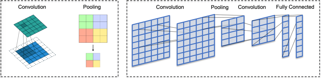
Convolutional Neural Networks (CNNs)
A method which takes words or phrases and creates higher level features from them. These features can then be used downstream as word/phrase embeddings. While they can be fairly effective, they are not good as other Deep Learning methods at ascribing meaning based on short or long distance contextual information. Most of the time CNN output is taken downstream to aid other NLP classifiers. Below is a diagram covering the salient components of a CNN – namely convolution and pooling.
For more information on CNNs, check out this guide.
Recurrent Neural Networks (RNNs)
Recurrent Neural Networks essentially models sequential data and is able to comprehend the past and the present of the inputs. This makes them very powerful for text prediction or generation, however they suffer from the vanishing gradient problem where the back-propagation gradients (important artifacts that help the network learn) get closer and closer to 0 with the more layers that the network has. There are variants of RNNs that can prevent this from happening, namely LSTMs, GRUs, and ResNets. They generally work by having input, output, and forget gates that can help bring in relevant data, and drop-out irrelevant data. Another issue of RNNs is the notion that they take a long time to train, and Attention Mechanism architectures such as Transformers aim to solve this problem. Below is a rough diagram describing the general architecture of RNNs.

For more information on RNNs, check out this guide.
Attention Mechanism
An idea that expands upon RNNs and their more complex LSTM/GRU counterparts. The idea is that as the nerual net learns from the data, it pays attention to only relevant features, words, or phrases that are important for the task at hand. Transformers use this notion of attention in the form of data matrices and combines a seq2seq model (which typically has an input, a decoder, and an output). First the data is taken in as input and attention is applied at some point between the input and the output, so that when generating the output it is typically higher quality as the attention model has tuned for what is relevant. For more information on Transformers, and this class of architectures, check out this resource.
Additionally, for a deeper guide on Deep Learning methods for NLP, you can check out this guide (Deep Learning for NLP: An Overview of Recent Trends)
Few Shot Learning
All of the NLP examples we described previously assumed that we have plenty of labeled data to work with. What if, however, we only have a few labeled examples (a handful, or a dozen, or a hundred). If it is easy and inexpensive to label more data, that would be the advised solution. However, if we don’t have such luxuries we have to use Zero/One Shot Learning or Few Shot Learning.
Zero Shot Learning
Zero Shot Learning in the NLP community refers to using an algorithm to classify things it wasn’t trained to classify in the first place. This is a complex topic to explain and this article by Joe Davidson does a great job.
One Shot Learning
One Shot Learning as the name implies is a framework that can create a decent classifier based on one data point. This may not apply as much in NLP as it has traditionally been used in the Computer Vision community. Though there is definitely some good experimental work at the moment that is applying One Shot Learning to NLP.
Few Shot Learning
Few Shot Learning is more relevant to NLP as it allows for using the few labeled samples that we have to create classifiers that can either be good-enough based on some evaluation metric, or fairly poor, but still be relevant enough to label more of our data. Once we have more of our data labeled with those rough labels, we can then create better NLP algorithms, and with enough hyper-parameter tuning and the right regularizers/loss-functions – one should be able to have generally good results at the end of this process.
For more information on how these approaches work, see the following resources:
Text classification from few training examples – Maël Fabien
Evaluating Our Classifiers
Okay so we just built some NLP models to do our bidding, and now how do we know how well they perform? There are a few widely used metrics that come to mind here. It also helps to have an example to frame our thoughts. Let’s say we built a classifier that can detect someone’s mood based on their writing. The options in this simple example are: cheerful, sad, angry, and humorous.
We then train our classifier on our training set, and have another set of data called the test set which the classifier was not trained on but which we labeled ourselves for evaluation purposes. Sometimes the test set can also be referred to as the development set, and the distinction between them is the following. The development set can be used internally while training the model with different configurations, features, hyper-parameters, etc., while the test set is then used at the end for one final check once the training is done. Both the development and test sets are labeled sets of data where we have text sections annotated with the writer’s mood.
We run the classifier on the test set and compute the following:
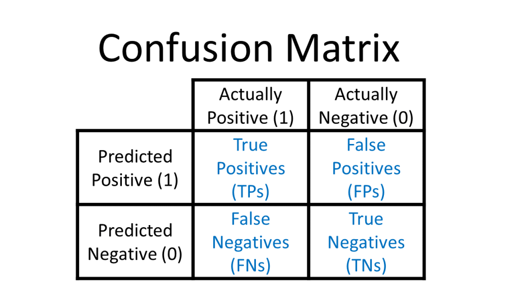
True Positives – For a given class (or mood in this case) we count the number of times the NLP classifier predicted that the given class was the true class. (e.g. for class “happy”: Truth = “happy” / Predicted = “happy”)
True Negatives – For a given class (or mood in this case) we count the number of times the NLP classifier did not predict that class, and indeed, the true class was not that class. (e.g. for class “happy”: Truth = “sad” / Predicted = “humorous”)
False Positives – For a given class (or mood in this case) we count the number of times the NLP classifier predicts an incorrect class which is different from the truth. (e.g. for class “happy”: Truth = “sad” / Predicted = “happy”)
False Negatives – For a given class (or mood in this case) we count the number of times the NLP classifier predicts that a data point does not belong to a class, but it does in the ground truth data. (e.g. for class “happy”: Truth = “happy” / Predicted = “sad”)
Most Data Science teams refer to these metrics in one simple concept called the Confusion Matrix as illustrated below, and there are many code libraries in every Data Science programming language that can easily compute this matrix, and these metrics for you.
Now that we have the confusion matrix, we can easily compute more interpretable metrics such as accuracy, precision, recall, and F-Score.
Accuracy – The percentage of correct predictions. A simple metric that can tell us how well our classifier is doing, but does not work very well with imbalanced data. For instance, if the class of “happy” had 10 data points, and the class of “sad” had 10,000 data points, then this metric would yield obscuring results which are not useful.
Formulas
accuracy = correct predictions / all predictions
Or
accuracy = (true positives + true negatives) / (true positives + true negatives + false positives + false negatives)
Precision – Of all the data points that were labeled a certain class, the percentage of them that were labeled successfully.
Formula
precision = true positives / (true positives + false positives)
Recall – Of all the data points that should have been labeled a certain class, the percentage of them that were labeled that class.
Formula
recall = true positives / (true positives + false negatives)
Accuracy was great because it provided us one true number to go by, and now we have to deal with two extra metrics? Not to worry, we have this covered with the F-Score.
F1 – Known as the harmonic mean of precision and recall, it combines these two metrics where an F1 score of 1 is perfect Precision/Recall, while anything less than that is not perfect. While this grately varies depening on the task at hand, an F1 score between 0.7 – 1 is considered pretty good. There are also many variations of the F-score that put emphasis on different things (e.g. puts more emphasis on the Precision or Recall).
Formula
F1 = 2 * (precision * recall) / (precision + recall)
For more information on evaluating machine learning models, check out this post.
There is also the notion of bias, variance, underfitting, and underfitting. Here is how they are related.
Bias – When a classifier makes assumptions about the data and misses the mark in prediction, likely because it was not trained with the right functions that can map the relationships between our data. For a classifier that has high bias, we can say that it underfit to our data.
Variance – When a model’s classifications are different from each other, likely this is because the model has overfit to the training data, and is not able to hit the mark as well on the test data.
These issues can be used by either training different models and using different functions to better model our data, or using regularizers.
For a great resource on the bias-variance trade-off, which is a known concept in Machine Learning, check this article out by Jason Brownlee
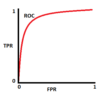
Finally, there is the AUC measure or ROC curve which measure how well your classifier can separate between classes. Typically an AUC close to 1 means that your classifier can distinguish between your classes perfectly. This resembles a plot similar to this one:
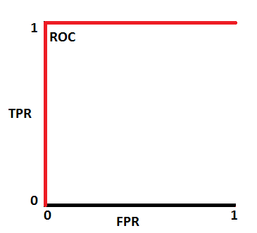
While, in general, most good classifiers are in the 0.7 – 1 range which look something more like this:
A great resource that explains AUC/ROC in depth can be found here – Understanding AUC – ROC Curve by Sarang Narkhede
Popular Frameworks, Libraries, and Places to Visit in the NLP World
If you want to create NLP classifiers, taking a course may help you cover the theory, but what then? It is very time-consuming to create tokenizers, algorithms, preprocessors, learners, transformers, evaluators from scratch – unless you really want to understand the internals for practice. Most of the time it is advised to use tried-and-tested libraries and frameworks. Below are some very useful NLP frameworks at the moment:
TensorFlow, PyTorch, and Keras – State-of-the art frameworks to help you build Deep Learning classifiers for NLP. While PyTorch gives a lot of granularity and control given the finest of details, it has a steeper learning curve. In contrast, TensorFlow is the easiest to use, with simple abstractions to help you focus more on the classifiers and less on the theory/implementation. Keras is the middle-ground between the two. Pick your tool of choice based on the time you have and what your project requires as all three are popular.
SpaCy – If you quickly want to build NLP code that works blazingly fast in production
NLTK – A great tool for learning about and exploring NLP problems, and sometimes doing research
Scikit-learn – Great resource for supervised / unsupervised learning and general ML
Huggingface – The place to be if you want to build transformers
Gensim – A very powerful library for topic modeling and text similarity analytics
CoreNLP – Your hero if you want to build NLP with Java
Amazon Mechanical Turk – A cheap and scalable solution to labeling NLP data
Resources for Tuning/Optimization
Tools for DevOps and NLP in production
For more such tools see the following articles.
Learning Resources
There are many resources to learn about NLP depending on what level of expertise you have. There are courses, books, GitHub repositories, blogs, and publications you can study. A great resource that explains all of it is this blog post:
The quickest way to learn in my opinion is to learn by doing by following the contents this free repository by fastai – (course-nlp)
Alternatively, if you’re a more advanced NLP practitioner and want to keep up to date with the latest and greatest findings in NLP, subscribing to Arxiv’s Computation and Language news/RSS feed will allow you to read the most recent publications in the field, thus, taking you to the edge of knowledge on this topic.
Conclusion
That’s all folks! I hope that this guide will help someone who wants to understand how to apply NLP techniques to solve their text analytics problems. Cheers, and Huggingface emojis to all of you. 🤗
